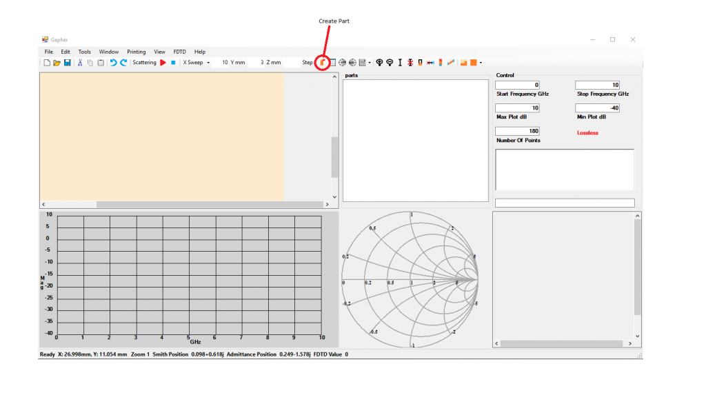
To match a device to the characteristic impedance of the circuit click on the Create part in the Home Window Figure 1.

Creating the parts

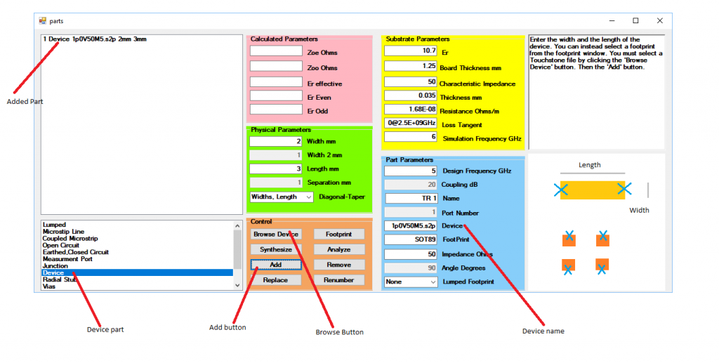
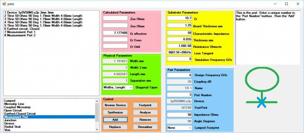
Select the Parts Window. In the Parts Window select the Device in the parts list window and then click on the Browse Device button, Figure 2.

This will open an Open Device Window so that an S parameter file can be selected. This file must be an s2p file. Here the BFP405 from Infineon Technology VCE = 0.5 V, IC = 0.5 mA Common Emitter S-Parameters is used, 1p0V50M5.s2p. Select the s2p file and click the Add button to place the part in the Parts Window as in Figure 2.

Now fill in the parameters of the board in the Substrate Parameters, the yellow section. Select the microstrip line in the Parts List. In the Part Parameters, the blue section, fill in the Design Frequency, Impedance and Angle of the microstrip line. 6 GHz Design Frequency, 50 Ohms Impedance and 90 degrees Angle are used here. The Design Frequency is the frequency that the microstrip lines will be designed. This can be independent of the Simulation Frequency. Click on the Synthesize button then click the Add button four times to add four of these to the Parts Window. An earth is required so select the Earthed, Closed Circuit, in the Parts List and then the Add button. Two ports are also required. Select the Measurement Port in the Parts List and then click the Add button twice to add two ports to the Parts Window. Enter the board parameters into the Substrate Parameter section, the yellow section and set the Simulation Frequency to 6GHz as in Figure 3, this will be the simulation frequency for the Component Sweep, and close the Parts Window. Finally add a 50 Ohm 2mm by 3mm Lumped resistor to the parts.

Calculating the input and output impedances

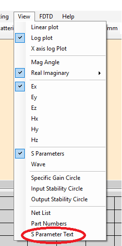
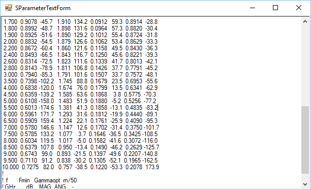
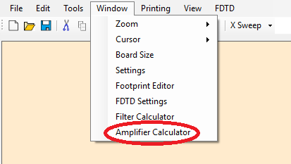
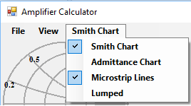
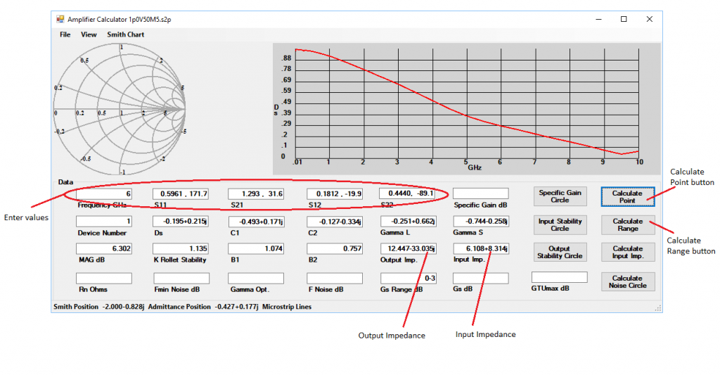
The matching input and output impedances need to be calculated. There are two ways of doing this. Using the Calculate Point button. In the Home Window select the device in the Parts Box to select the device and then click on the S Parameter Text in the View Menu, Figure 3. This will bring up a new Window with the Touchstone format text of the S parameters, Figure 4. Open the Amplifier Calculator in View Menu of the Home Window, Figure 5, to bring up the Amplifier Window, Figure 7. Select the Microstrip Lines from the Smith Menu, Figure 6. Enter the values for the Frequency, S11, S12, S21 and S22, here the values of frequency “6”, S11 “0.5961 , 171.7”, S21 “1.293 , 31.6”, S12 “0.1812 , -19.9” and S22 “0.4440, -89.1” remembering to put a comma between the magnitude and the angle and click the Calculate Point button. The values will then be calculated Figure 7. Double click on the Input Impedance textbox and this will send the part to the Parts Window in the Home Window. Similarly double click on the Output Impedance to send this to the Parts Window.

2. Using the Calculate Range button. In the Home Window select the device in the Parts Box and then open the Amplifier Calculator in View Menu of the Home Window, Figure 5. Select the Microstrip Lines from the Smith Menu, Figure 6. Now click on the Calculate Range button. Click on the Plot Window and drag the mouse while in the Plot Window. A white cursor will appear. This will update all the values in the textboxes at the cursor position. When the cursor is at the desired frequency click the left mouse button to clear the cursor and freeze the values in the textboxes. Double click on the Input Impedance textbox and this will send the part to the Parts Window in the Home Window. Similarly double click on the Output Impedance to send this to the Parts Window.

Figure 6 Selecting the non conjugate impedances

Figure 7 the Amplifier calculator for the transistor

The input impedance on the Smith chart

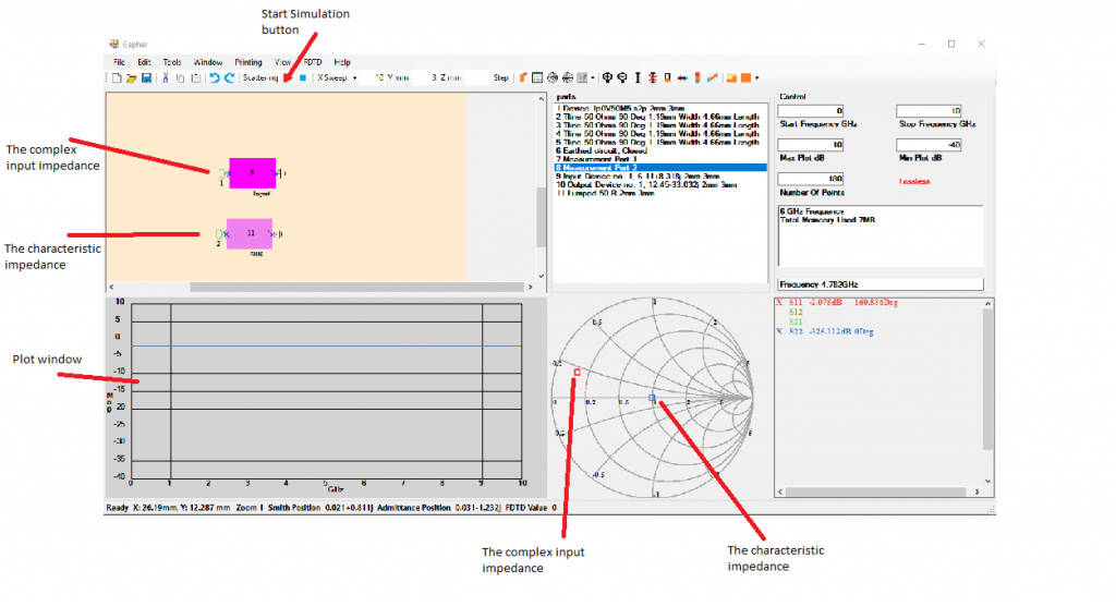
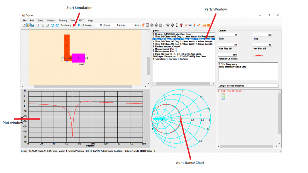
Starting with the Input Impedance, part 9, place it in the Circuit Window and put Port 1, part 7, to the left of it and an Earth, part 6, to the right. Place the 50 Ohm Resistor, part 11, in the Circuit Window and place Port 2, part 7, to the left of it and an Earth, part 6, to the right. Set the Start Frequency to 0 GHz, the Stop Frequency to 10 GHz and the Number of points to 40 and click the Start Simulation button. Now left click in the Plot Window. The complex input impedance and the characteristic impedance, here it’s 50 Ohms, are plotted on the Smith chart in Figure 8. The two impedances will have to be connected using microstrip lines so that the input impedance sees itself and the characteristic impedance sees 50 Ohms.

Matching the input port

Make sure Gapher is in the S Parameter mode, FDTD in the FDTD menu is unchecked and in the View menu the Real Imaginary is checked with the Admittance checked too. Using the parts numbered 9 Input, 6 Earth, 2 Microstrip Line and 7 Port 1 create the circuit in Figure 56. Click on the following, the S11 plot variable, click on the down arrow next to the Sweep type icon and select the Component Sweep. Click the Admittance Chart button and the Smith Chart button so that only the Admittance chart is visible. Click on part 2 in the Parts Window, this is the part to be swept. In the Control section the start, stop and number of points to plot values can be changed. Here they have been set to 0, 180 and 180 respectfully. And then click on the Start Simulation button. Left click in the Plot Window and drag the mouse so that the cursor in the Smith window is on the point that crosses the 1 circle as in Figure 9. When Admittance in the View, Real Imaginary Menu is checked the output in the Plot Variable window will be the admittance, then the Real part in the Plot Variable will be close to 50 Ohms.

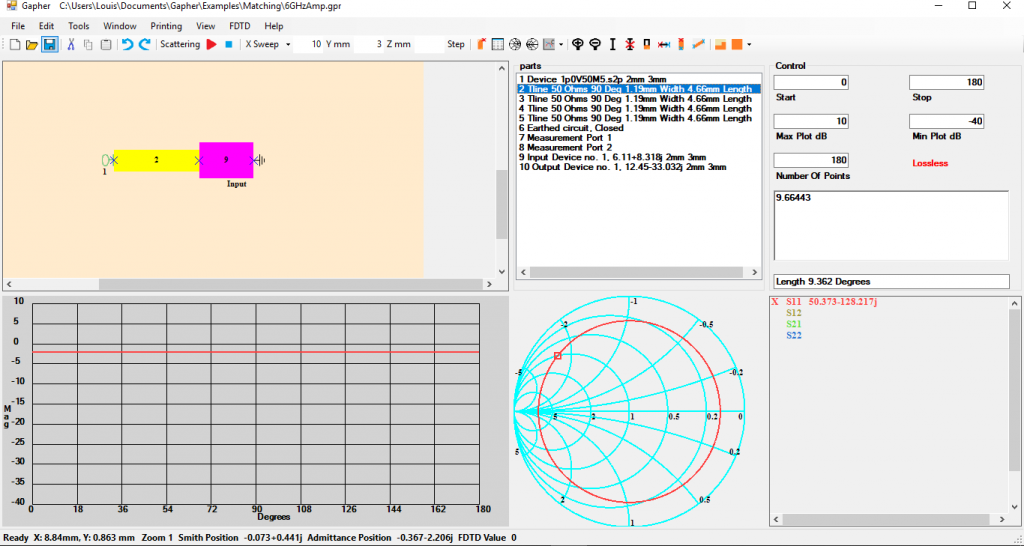
Figure 9 matching the input with the first microstrip line

Now right click while in the Plot Window. Part 2 will disappear and the cursor will be a shorter length microstrip line with the value of the length being displayed in the Parts Box. Using this part place join it as it was before onto the left of part 9. Select part 3 in the Parts Box and right click in the Circuit Window to rotate it vertical and join that to the left side of part 2. Now either press the escape keyboard button or click on the Cursor Off button to hide the cursor. Right click on the Port in the Circuit Window to pick it up and join that to the left of the Junction, as in Figure 10.

Select part 3 In the Parts Box to select the part to be swept. Click on the Start Simulation button to run the simulation. Left click in the Plot Window and drag the mouse until the cursor in the Smith Chart on the 1 circle is on the horizontal line as in Figure 57. Right click while in the Plot Window. Part 3 disappears and the cursor is replaced by a shorter length microstrip line. Join this to the junction top as it was before.

Figure 10 matching the input with the second microstrip line

The output impedance on the Smith chart

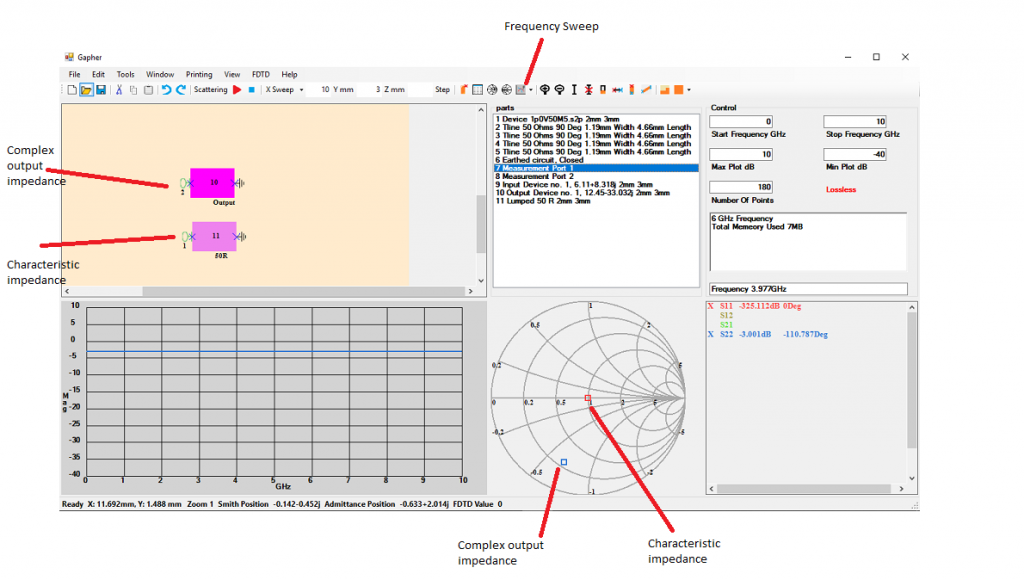
Starting with the Output Impedance, part 10, place it in the Circuit Window and put Port 1, part 7, to the left of it and an Earth, part 6, to the right. Place the 50 Ohm Resistor, part 11, in the Circuit Window and place Port 2, part 7, to the left of it and an Earth, part 6, to the right. Select Frequency Sweep and run the simulation. Click in the Plot Window and the output and characteristic impedances are plotted on the Smith chart in Figure 11. These will have to be joined using microstrip lines to match them to each other. Now select the Component Sweep.

Matching the output port

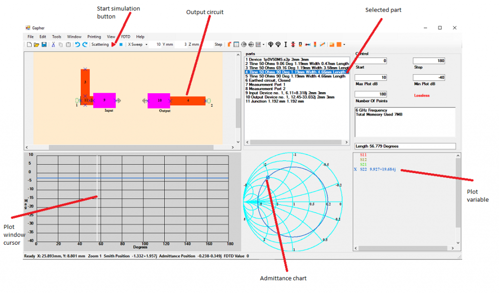
Now for the output port, using the parts 4, 6, 8 and 10 create the circuit in Figure 12. In the Port Variable Window deselect S11 and select S22 as the plot variable. Select part 4, the 3^rd microstrip line, in the Parts Box to make it the sweep variable. Stay in Component Sweep mode and keep the Admittance chart. Start the simulation. If the cursor in the Plot Window is not visible left click in the Plot window to bring up the cursor. Drag the mouse so that the cursor in the Admittance chart crosses the 1 circle as in Figure 12, in the Plot Variable window this will be about 50 Ohms if Admittance is selected in the View, Real Imaginary Admittance is checked, then right click. The part will disappear from the circuit and become a cursor with the required length. Place that part as it was before on the output part.

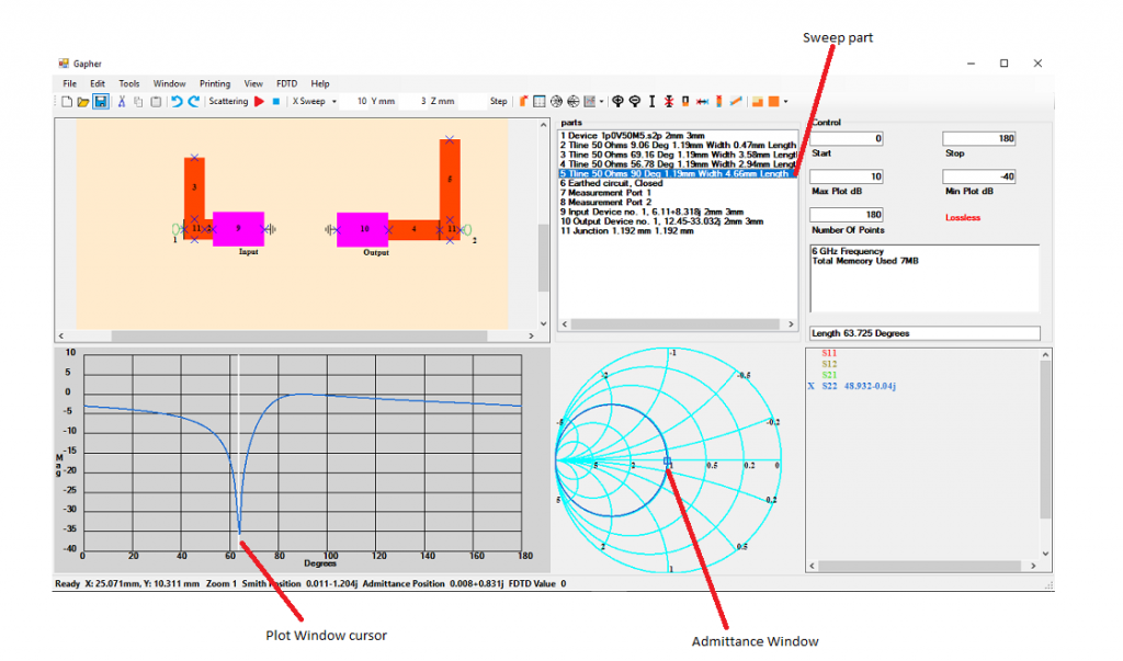
Select part 5, the 4^th microstrip line, and right click in the Circuit Window to rotate the part vertically. Place the bottom of this part to the right of part 4 as in Figure 13. Select part 5 in the Parts Box and run the simulation. Drag the mouse in the Plot Window so that the cursor in the Admittance Chart is on the horizontal line where the 1 circle cuts it and right click. Join the part as it was before which should look like Figure 13.

Figure 13 matching the output port with the 4th microstrip line

Joining the input and output matched circuits together of the 6GHz amplifier

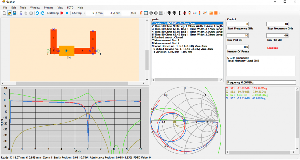
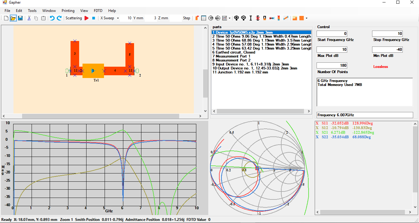
Remove parts 9, 10 and the two Earths. Select part 1, the device, and join that to the right of the part 2. Click on the Cut button and cut all of the right circuit. Click on the Paste button and paste it to the right of the device, as in Figure 14.

Select all the parameters in Plot Variables. Select the Frequency Sweep, from the Sweep Type button, turn on the Smith Chart and off the Admittance Chart and start the simulation. The Plot Window will now display the results and show that the amplifier is matched at 6 GHz, Figure 14. By left clicking on the plot window and dragging the mouse the values of the parameters will be displayed in the Plot Variables window.